Data scientists, according to interviews and expert estimates, spend from 50 percent to 80 percent of their time mired in this more mundane labor of collecting and preparing unruly digital data, before it can be explored for useful nuggets.
– “For Big-Data Scientists, ‘Janitor Work’ Is Key Hurdle to Insight” (New York Times, 2014)
janitor has simple functions for examining and cleaning dirty data. It was built with beginning and intermediate R users in mind and is optimized for user-friendliness. Advanced R users can perform many of these tasks already, but with janitor they can do it faster and save their thinking for the fun stuff.
The main janitor functions:
- perfectly format data.frame column names;
- create and format frequency tables of one, two, or three variables - think an improved
table(); and - provide other tools for cleaning and examining data.frames.
The tabulate-and-report functions approximate popular features of SPSS and Microsoft Excel.
janitor is a #tidyverse-oriented package. Specifically, it plays nicely with the %>% pipe and is optimized for cleaning data brought in with the readr and readxl packages.
Installation
You can install:
- the most recent officially-released version from CRAN with
install.packages("janitor")- the latest development version from GitHub with
# install.packages("remotes")
remotes::install_github("sfirke/janitor")
# or from r-universe
install.packages("janitor", repos = c("https://sfirke.r-universe.dev", "https://cloud.r-project.org"))
Using janitor
A full description of each function, organized by topic, can be found in janitor’s catalog of functions vignette. There you will find functions not mentioned in this README, like compare_df_cols() which provides a summary of differences in column names and types when given a set of data.frames.
Below are quick examples of how janitor tools are commonly used.
Cleaning dirty data
Take this roster of teachers at a fictional American high school, stored in the Microsoft Excel file dirty_data.xlsx: 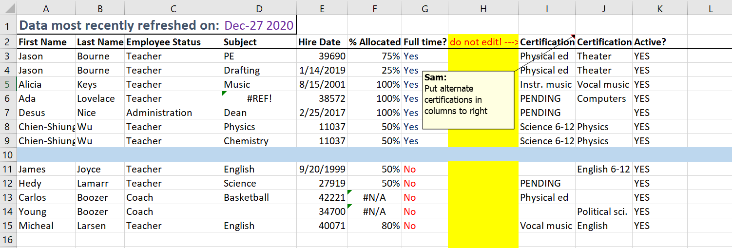
Dirtiness includes:
- A header at the top
- Dreadful column names
- Rows and columns containing Excel formatting but no data
- Dates in two different formats in a single column (MM/DD/YYYY and numbers)
- Values spread inconsistently over the “Certification” columns
Here’s that data after being read in to R:
library(readxl)
library(janitor)
library(dplyr)
library(here)

roster_raw <- read_excel(here("dirty_data.xlsx")) # available at https://github.com/sfirke/janitor
glimpse(roster_raw)
#> Rows: 14
#> Columns: 11
#> $ `Data most recently refreshed on:` <chr> "First Name", "Jason", "Jason", "Alicia", "Ada", "Desus", "Chien-…
#> $ ...2                               <chr> "Last Name", "Bourne", "Bourne", "Keys", "Lovelace", "Nice", "Wu"…
#> $ ...3                               <chr> "Employee Status", "Teacher", "Teacher", "Teacher", "Teacher", "A…
#> $ `Dec-27 2020`                      <chr> "Subject", "PE", "Drafting", "Music", NA, "Dean", "Physics", "Che…
#> $ ...5                               <chr> "Hire Date", "39690", "43479", "37118", "38572", "42791", "11037"…
#> $ ...6                               <chr> "% Allocated", "0.75", "0.25", "1", "1", "1", "0.5", "0.5", NA, "…
#> $ ...7                               <chr> "Full time?", "Yes", "Yes", "Yes", "Yes", "Yes", "Yes", "Yes", NA…
#> $ ...8                               <chr> "do not edit! --->", NA, NA, NA, NA, NA, NA, NA, NA, NA, NA, NA, …
#> $ ...9                               <chr> "Certification", "Physical ed", "Physical ed", "Instr. music", "P…
#> $ ...10                              <chr> "Certification", "Theater", "Theater", "Vocal music", "Computers"…
#> $ ...11                              <chr> "Active?", "YES", "YES", "YES", "YES", "YES", "YES", "YES", NA, "…
Now, to clean it up, starting with the column names.
Name cleaning comes in two flavors. make_clean_names() operates on character vectors and can be used during data import:
roster_raw_cleaner <- read_excel(here("dirty_data.xlsx"),
  skip = 1,
  .name_repair = make_clean_names
)
glimpse(roster_raw_cleaner)
#> Rows: 13
#> Columns: 11
#> $ first_name        <chr> "Jason", "Jason", "Alicia", "Ada", "Desus", "Chien-Shiung", "Chien-Shiung", NA, "J…
#> $ last_name         <chr> "Bourne", "Bourne", "Keys", "Lovelace", "Nice", "Wu", "Wu", NA, "Joyce", "Lamarr",…
#> $ employee_status   <chr> "Teacher", "Teacher", "Teacher", "Teacher", "Administration", "Teacher", "Teacher"…
#> $ subject           <chr> "PE", "Drafting", "Music", NA, "Dean", "Physics", "Chemistry", NA, "English", "Sci…
#> $ hire_date         <dbl> 39690, 43479, 37118, 38572, 42791, 11037, 11037, NA, 36423, 27919, 42221, 34700, 4…
#> $ percent_allocated <dbl> 0.75, 0.25, 1.00, 1.00, 1.00, 0.50, 0.50, NA, 0.50, 0.50, NA, NA, 0.80
#> $ full_time         <chr> "Yes", "Yes", "Yes", "Yes", "Yes", "Yes", "Yes", NA, "No", "No", "No", "No", "No"
#> $ do_not_edit       <lgl> NA, NA, NA, NA, NA, NA, NA, NA, NA, NA, NA, NA, NA
#> $ certification     <chr> "Physical ed", "Physical ed", "Instr. music", "PENDING", "PENDING", "Science 6-12"…
#> $ certification_2   <chr> "Theater", "Theater", "Vocal music", "Computers", NA, "Physics", "Physics", NA, "E…
#> $ active            <chr> "YES", "YES", "YES", "YES", "YES", "YES", "YES", NA, "YES", "YES", "YES", "YES", "…
clean_names() is a convenience version of make_clean_names() that can be used for piped data.frame workflows. The equivalent steps with clean_names() would be:
roster_raw <- roster_raw %>%
  row_to_names(row_number = 1) %>%
  clean_names()
The data.frame now has clean names. Let’s tidy it up further:
roster <- roster_raw %>%
  remove_empty(c("rows", "cols")) %>%
  remove_constant(na.rm = TRUE, quiet = FALSE) %>% # remove the column of all "Yes" values
  mutate(
    hire_date = convert_to_date(
      hire_date, # handle the mixed-format dates
      character_fun = lubridate::mdy
    ),
    cert = dplyr::coalesce(certification, certification_2)
  ) %>%
  select(-certification, -certification_2) # drop unwanted columns
#> Removing 1 constant columns of 10 columns total (Removed: active).

roster
#> # A tibble: 12 × 8
#>    first_name   last_name employee_status subject    hire_date  percent_allocated full_time cert
#>    <chr>        <chr>     <chr>           <chr>      <date>     <chr>             <chr>     <chr>
#>  1 Jason        Bourne    Teacher         PE         2008-08-30 0.75              Yes       Physical ed
#>  2 Jason        Bourne    Teacher         Drafting   2019-01-14 0.25              Yes       Physical ed
#>  3 Alicia       Keys      Teacher         Music      2001-08-15 1                 Yes       Instr. music
#>  4 Ada          Lovelace  Teacher         <NA>       2005-08-08 1                 Yes       PENDING
#>  5 Desus        Nice      Administration  Dean       2017-02-25 1                 Yes       PENDING
#>  6 Chien-Shiung Wu        Teacher         Physics    1930-03-20 0.5               Yes       Science 6-12
#>  7 Chien-Shiung Wu        Teacher         Chemistry  1930-03-20 0.5               Yes       Science 6-12
#>  8 James        Joyce     Teacher         English    1999-09-20 0.5               No        English 6-12
#>  9 Hedy         Lamarr    Teacher         Science    1976-06-08 0.5               No        PENDING
#> 10 Carlos       Boozer    Coach           Basketball 2015-08-05 <NA>              No        Physical ed
#> 11 Young        Boozer    Coach           <NA>       1995-01-01 <NA>              No        Political sci.
#> 12 Micheal      Larsen    Teacher         English    2009-09-15 0.8               No        Vocal music
Examining dirty data
Finding duplicates
Use get_dupes() to identify and examine duplicate records during data cleaning. Let’s see if any teachers are listed more than once:
roster %>% get_dupes(contains("name"))
#> # A tibble: 4 × 9
#>   first_name   last_name dupe_count employee_status subject   hire_date  percent_allocated full_time cert
#>   <chr>        <chr>          <int> <chr>           <chr>     <date>     <chr>             <chr>     <chr>
#> 1 Chien-Shiung Wu                 2 Teacher         Physics   1930-03-20 0.5               Yes       Science …
#> 2 Chien-Shiung Wu                 2 Teacher         Chemistry 1930-03-20 0.5               Yes       Science …
#> 3 Jason        Bourne             2 Teacher         PE        2008-08-30 0.75              Yes       Physical…
#> 4 Jason        Bourne             2 Teacher         Drafting  2019-01-14 0.25              Yes       Physical…
Yes, some teachers appear twice. We ought to address this before counting employees.
Tabulating tools
A variable (or combinations of two or three variables) can be tabulated with tabyl(). The resulting data.frame can be tweaked and formatted with the suite of adorn_ functions for quick analysis and printing of pretty results in a report. adorn_ functions can be helpful with non-tabyls, too.
tabyl()
Like table(), but pipe-able, data.frame-based, and fully featured.
tabyl() can be called two ways:
- On a vector, when tabulating a single variable:
tabyl(roster$subject) - On a data.frame, specifying 1, 2, or 3 variable names to tabulate:
roster %>% tabyl(subject, employee_status).- Here the data.frame is passed in with the
%>%pipe; this allowstabylto be used in an analysis pipeline
- Here the data.frame is passed in with the
One variable:
roster %>%
  tabyl(subject)
#>     subject n    percent valid_percent
#>  Basketball 1 0.08333333           0.1
#>   Chemistry 1 0.08333333           0.1
#>        Dean 1 0.08333333           0.1
#>    Drafting 1 0.08333333           0.1
#>     English 2 0.16666667           0.2
#>       Music 1 0.08333333           0.1
#>          PE 1 0.08333333           0.1
#>     Physics 1 0.08333333           0.1
#>     Science 1 0.08333333           0.1
#>        <NA> 2 0.16666667            NA
Two variables:
roster %>%
  filter(hire_date > as.Date("1950-01-01")) %>%
  tabyl(employee_status, full_time)
#>  employee_status No Yes
#>   Administration  0   1
#>            Coach  2   0
#>          Teacher  3   4
Three variables:
roster %>%
  tabyl(full_time, subject, employee_status, show_missing_levels = FALSE)
#> $Administration
#>  full_time Dean
#>        Yes    1
#>
#> $Coach
#>  full_time Basketball NA_
#>         No          1   1
#>
#> $Teacher
#>  full_time Chemistry Drafting English Music PE Physics Science NA_
#>         No         0        0       2     0  0       0       1   0
#>        Yes         1        1       0     1  1       1       0   1
Adorning tabyls
The adorn_ functions dress up the results of these tabulation calls for fast, basic reporting. Here are some of the functions that augment a summary table for reporting:
roster %>%
  tabyl(employee_status, full_time) %>%
  adorn_totals("row") %>%
  adorn_percentages("row") %>%
  adorn_pct_formatting() %>%
  adorn_ns() %>%
  adorn_title("combined")
#>  employee_status/full_time         No        Yes
#>             Administration   0.0% (0) 100.0% (1)
#>                      Coach 100.0% (2)   0.0% (0)
#>                    Teacher  33.3% (3)  66.7% (6)
#>                      Total  41.7% (5)  58.3% (7)
Pipe that right into knitr::kable() in your RMarkdown report.
These modular adornments can be layered to reduce R’s deficit against Excel and SPSS when it comes to quick, informative counts. Learn more about tabyl() and the adorn_ functions from the tabyls vignette.
Contact me
You are welcome to:
- submit suggestions and report bugs: https://github.com/sfirke/janitor/issues
- let me know what you think on Mastodon: @samfirke@a2mi.social
- compose a friendly e-mail to: